We’ve made some improvements to Hierarqcal since its initial release last year. I hope to summarise the notable ones in this post and give some examples. The biggest change of all being a new logo:

But, there are other changes too, we have:

• New Tutorials
  • Grover’s Algorithm, thanks to @AmyRouillard
  • The Quantum Fourier Transform, thanks to @AmyRouillard
  • VQE of Hydrogen Molecule, thanks to @Gopal-Dahale
• Core Functionality Improvements
  • General compute graph generation
  • A new Qpivot primitive thanks to @AmyRouillard
  • Reworked the Qmask primitive
  • Functionality to parametrise gates based on functional relationships
• User Interface Improvements
  • A new plot_circuit function to visualise abstract circuits
  • New plotting functions for visualising hypergraphs thanks to @metalcyanide
  • The ability to generate qiskit circuits with strings thanks to @khnikhil
• Research
  • Overview of the representation and application to Quantum Phase Recognition
  • Application in generating circuits for pulsar classification

For a quick overview, I’ll share these interactive slides which was presented at unitaryCON and QTML 2023. It showcases a lot of the new functionality and provides some step by step examples (select the frame and use up, down, left and right arrows). If you’re interested, you can find the full set of slides online.

A brief walk through the new stuff

At its core HierarQcal is a tool to generate compute graphs. It leverages a hierarchical representation to enable both user and machine to design these graphs in a modular and (unsurprisingly) hierarchical way. For example, when “designing” an algorithm for multiplication we use “units” of addition repeated in some pattern. That unit of addition consists of “units” of adders which themselves consists of “units” of logic gates, such as “and” or “or”. HierarQcal provides an interface to work on these different levels, so that a machine for example, can create their own units and use them to build higher level units (motifs). The highest level unit is then the algorithm it designed.

For example, hierarqcal may be used to generate ansatzes for quantum algorithms, such as the Variational Quantum Eigensolver (VQE). It is also possible to generate Quantum Convolutional Neural Networks (QCNNs) for Quantum Phase Recognition (QPR) as demonstrated in our recent paper. There we utilise an evolutionary algorithm to apply the above ideas for classifying quantum phases of matter. The modular and hierarchical nature of the representation compliments evolutionary algorithms, where your units are “genotypes” that mutate and combine to form more complicated units. Below we show a simple example of such an algorithm, it consists of the following steps:

1. Initialise a population of random circuits (primitive cells)
2. Select a subset of the population (tournament selection)
3. From the subset, gather the top two performing circuits
4. Mutate each of the top two performing circuits to create two new circuits
5. Combine (join) the top two performing circuits to create one new circuit
6. Throw the 3 new circuits into the population, along with the original two
7. Repeat step 1-6 until some stopping condition is met

To facilitate more general compute graph generation we’ve added the ability to provide any python function as a mapping for motifs. These functions are of the form:

def generic_f(bits, symbols=None, state=None):
    pass

where state corresponds to some arbitrary object that gets passed around and is manipulated in the function, symbolscorrespond to any parameters that might be used to determine how the state changes and bits correspond to the specific indices of the state that is getting changed. In the case of a quantum circuit, bits would be the qubit labels, state would be the current state vector of the system and symbols could correspond to a list of angles which parametrise some rotational gates in the circuit. Calling a hierarchical motif i.e. my_motif(), executes these functions in order, the state gets changed and passed around until all operations are finished, then the state is returned at the end. For example, if for whatever reason you have a list of letters and want to concatenate all other letters to the first element, you could do:

from hierarqcal import Qpivot, Qinit, Qunitary

def concat(bits, symbols=None, state=None):
    state[bits[0]] += state[bits[1]]
    return state

first_8_letters = ["a", "b", "c", "d", "e", "f", "g", "h"]
give_0_more_letters = Qinit(8, state=first_8_letters) \
                    + Qpivot("1*", mapping=Qunitary(concat, 0, 2))
give_0_more_letters()
# output
['abcdefgh', 'b', 'c', 'd', 'e', 'f', 'g', 'h']

Note that the “algorithm” above is independent of list size, for larger lists only Qinit is changed accordingly (this just sets initial conditions) the abstract structure of the algorithm is captured in what follows after it, i.e. the Qpivot.Plotting the compute graph might help to see what’s going on:

from hierarqcal import plot_circuit
plot_circuit(give_0_more_letters)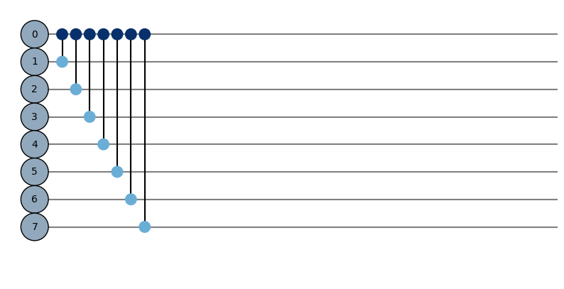

Here we are “pivoting” on the first bit, as was specified with the string "1*" in the Qpivot primitive. Within this pivot pattern 1*, the * character is shorthand for “fill the rest with zeroes”. Alternatively, we could have provided the explicit pivot pattern “10000000”. Similarly, the ”!” character is used as shorthand for “fill the rest with ones”. Each index in the string corresponds to each bit in order (i.e. pivot_str[0] -> bits[0]). Each 1 in the string indicates a pivot on its corresponding bit. Each 0 indicates non-pivots, each of these gets paired with a pivot. Here are some examples of how changing the pivot pattern changes the output:

['a', 'b', 'c', 'd', 'e', 'f', 'g', 'habcdefg'] # *1
['a', 'b', 'c', 'd', 'ea', 'fb', 'gc', 'hd'] # *!
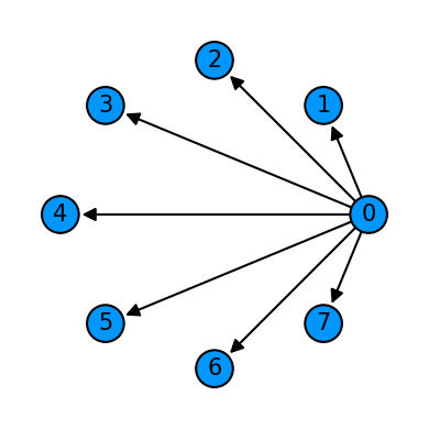
['a', 'b', 'c', 'dacg', 'ebfh', 'f', 'g', 'h'] # *11*

This example showcases the new Qpivot primitive and the abstract circuit plot_function. The Qpivot primitive splits the bits into two sets according to the ones and zeros in the pivot pattern. The elements of the first set, associated with “0”, are cycled through to pivot on the second set, associated with “1”. The digraph below shows this motif from another perspective:

Building your own quantum simulator for qubits, qutrits, qudits and so on, is then made easy since any python function can be provided to a motif. There’s multiple ways to achieve this, you can write functions that corresponds to gate operations and keep track of a tensor product that represents that state of the system. Another way would be to view the circuit as a tensor network and perform the correct tensor contractions. We’ve provided some functionality to facilitate this approach, for example below we show how to quickly see what a cycle of hadamards (one hadamard applied to each qubit) does to the |0…0> state.

import numpy as np
from hierarqcal import get_tensor_as_f, Qcycle, Qinit

n = 3
H_m = (1 / np.sqrt(2)) * np.array([[1, 1], [1, -1]])
H = Qunitary(get_tensor_as_f(H_m), 0, 1)

tensors = [np.array([1, 0], dtype=np.complex256)] * n
hierq = Qinit(n, tensors=tensors) + Qcycle(mapping=H)

print(hierq().flatten())
# Output
# [0.35355339+0.j 0.35355339+0.j 0.35355339+0.j 0.35355339+0.j
#  0.35355339+0.j 0.35355339+0.j 0.35355339+0.j 0.35355339+0.j]

The variable n can be increased to see the effect on more qubits (the use of Qcycle stays the same because it is independent of the number of qubits). The get_tensor_as_f helper function takes in a matrix and turns it into that generic function form. In the backend, tensor contraction is performed to compute the final state vector.

There is more, such as the rework of Qmask and its new relative Qunmask but for that I’ll refer you to the core functionality tutorial. Be sure to check it and the other tutorials out!

Future Directions

Currently, we’re working on extending the tensor network contraction functionality to include more general tensor networks, and to allow control over the contraction order. So far this representation has been useful in generating ansatzes for VQE, so there will be a focus on adding features to facilitate this. There is also work being done on symbolic manipulation of expressions with the aid of sympy. These expressions are represented as trees, and manipulating them corresponds to traversing parts of the tree and applying operations to its terms. With hierarqcal, it is convenient to specify bulk operations to specific parts of this tree. For example, applying commutation relations to a subset of fermionic/bosonic operators in a Hamiltonian of some quantum system. The way in which these operations are applied lend themselves to being captured by patterns similar to those seen in the Qpivot example.

That’s it for now!