Traditionally, creating quantum circuits requires specialized knowledge in quantum programming. This requirement holds true when encoding a classical algorithm inside a quantum circuit, for instance, for an oracle or a black-box component of a quantum algorithm. This often becomes a time wasting job, since we almost always already have a classical implementation in a traditional high level language.

Qlasskit, an open-source Python library developed with the support of a Unitary Fund microgrant, addresses this challenge head-on by allowing direct translation of standard Python code into invertible quantum circuits without any modification to the original code. Furthermore, qlasskit implements some well-known quantum algorithms and offers a comprehensive interface for implementing new ones.

Qlasskit adopts a distinctive method where it constructs a single boolean expression for each output qubit of the entire function, rather than translating individual operations into quantum circuits and then combining them. This approach enables advanced optimization by leveraging boolean algebraic properties.

For instance, let assume we have the following function:

from qlasskit import qlassf, Qint2, Qint4
from qiskit import QuantumCircuit

@qlassf
def f_comp(b: bool, n: Qint2) -> Qint2:
      for i in range(3):
            n += (1 if b else 2)
      return n

The first things you can notice in this code are:

• the qlassf decorators, indicating that the function will be translated to a quantum circuit.
• special bit-sized types Qint4, and Qint2. These are required as qubits are a precious resource, and we want to use as few as possible.
• it all reads as normal Python code.

If we decompose the algorithm in 3 separate additions and we compile them separately, we obtain the following circuit:

@qlassf
def f1(b: bool, n: Qint2) -> Qint2:
    return n + (1 if b else 2)

qc = QuantumCircuit(f_comp.num_qubits * 2 - 1)

for i in range(3):
    qc.append(f1.gate(), [0] + list(range(1 + i * 2, 5 + i * 2)))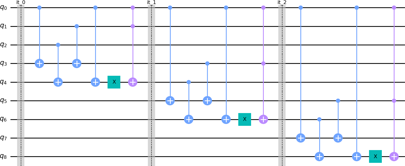

While if we compile the whole function to a quantum circuit using qlasskit, we obtain the following quantum circuit:

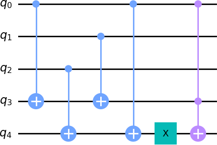
As we can see from the circuit drawings, qlasskit approach needs half the number of qubits and half the number of gates.

An use-case: pre-image attack on a cryptographic function

To further illustrate qlasskit’s capabilities, we will demonstrate its use in performing a pre-image attack on a cryptographic hash function using Grover’s search algorithm, obtaining a quadratic speedup compared to classical approaches. The beauty of qlasskit lies in its simplicity – you can write the entire software without needing to understand any concept of quantum computing.

A pre-image attack, in cryptography, targets a hash function h(m) with the aim to discover an original message m that corresponds to a specific hash value. On a traditional computer, to perform this attack without any hints, we must run h(m) with every possible input (N=2**n).

Thanks to the Grover search algorithm, we are able to find a pre-image with only pi/2 * sqrt(N) iterations, obtaining the quadratic speedup I mentioned before.

We write a toy hash function hash_simp which operates on messages composed of two 4 bit values and uses bitwise xor to create an 8 bit hash value.

from qlasskit import qlassf, Qint4, Qint8, Qlist

@qlassf
def hash_simp(m: Qlist[Qint4, 2]) -> Qint8:
    hv = 0
    for i in m:
        hv = ((hv << 4) ^ (hv >> 1) ^ i) & 0xff

    return hv

To see the resulting quantum circuit we can export and draw in qiskit:

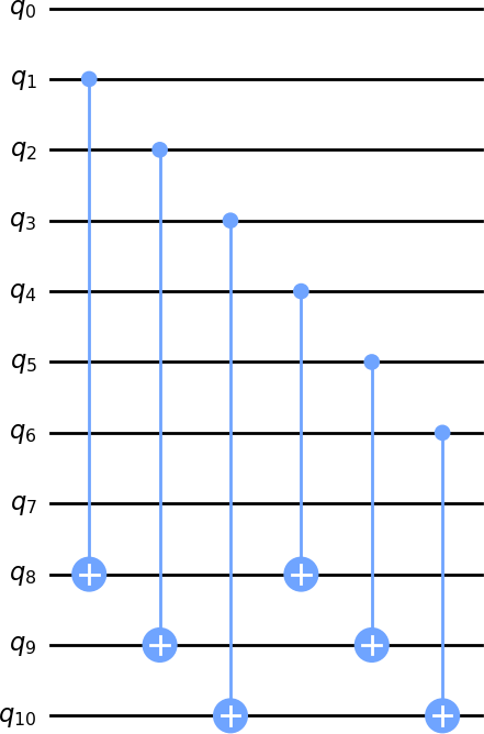
hash_simp.export('qiskit').draw('mpl')

And this is the resulting circuit, produced by the qlasskit internal compiler:

Thanks to the fact that qlasskit functions are standard Python functions, we can call the original_f to perform some kind of analysis and test on the hash function. Since the input space is tiny (it is a toy hash function), we can check if the hash function is uniform (if it maps equally to the output space).

from collections import Counter

d = Counter(hex(hash_simp.original_f((x, y))) for x in range(2**4) for y in range(2**4))

print('Hash function output space:', len(d))

We got that hash_simp is following an uniform distribution.

Now we use our quantum function as an oracle for a Grover search, in order to find which input maps to the value 0xca.

from qlasskit.algorithms import Grover

q_algo = Grover(hash_simp, Qint8(0xca))

Then we use our preferred framework and simulator for sampling the result; this is an example using qiskit with aer_simulator.

from qiskit import Aer, QuantumCircuit, transpile
from qiskit.visualization import plot_histogram

qc = q_algo.export('qiskit')
qc.measure_all()
simulator = Aer.get_backend("aer_simulator")
circ = transpile(qc, simulator)
result = simulator.run(circ).result()
counts = result.get_counts(circ)

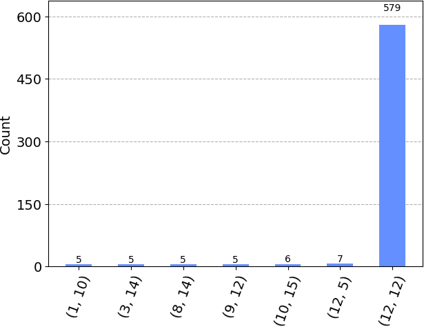
counts_readable = q_algo.decode_counts(counts, discard_lower=5)
plot_histogram(counts_readable)

And this is the result of the simulation, where we can see that the pre-image that leads to h(x) = 0xca is the list [12,12].

Using QlassF.original_f we can double check the result without invoking a quantum simulator; calling it with the list [12,12] must result in the hash value 0xca.

print(hex(hash_simp.original_f((12,12))))

A special thanks to the Unitary Fund that funded this idea. If you have any questions or comments, feel free to reach out to me on twitter dagide, linkedin Davide Gessa and medium @dakk.

Useful Links:

• Qlasskit library on github
• Qlasskit docs
• How qlasskit works