Qiskit is a popular choice among developers and researchers working in the field of quantum computing. It offers a wide range of functionalities and has useful extensions for algorithms, chemistry etc. On the other hand, Qulacs is known for its efficient quantum circuit simulation. Qiskit-Qulacs aims to act as a bridge between these two libraries. In this article, we’ll explore how the Qiskit-Qulacs offers users the best of both worlds.

The library is designed to make use of Qulacs’ fast simulation while abstracting it within Qiskit’s familiar environment. This allows users to create quantum circuits using Qiskit and execute them using Qulacs as the backend, resulting in faster circuit execution times for tasks like state vector simulations, calculating expectation values, and circuit gradient computations.

Getting Started

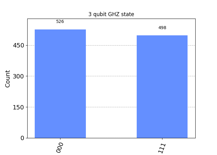
Let’s see how easy it is to use the Qiskit-Qulacs with a simple example. We create and run a 3-qubit GHZ state using Qiskit-Qulacs:

import matplotlib.pyplot as plt
from qiskit import QuantumCircuit
from qiskit.visualization import plot_histogram, plot_state_city

from qiskit_qulacs import QulacsProvider

# Create a bell state
qc = QuantumCircuit(3)
qc.h(0)
qc.cx(0, 1)
qc.cx(0, 2)

# Use Qiskit-Qulacs to run the circuit
backend = QulacsProvider().get_backend("qulacs_simulator")
result = backend.run(qc, shots=1024, seed_simulator=42).result()
counts = result.get_counts()

# Visualization
plot_histogram(counts)
plt.show()

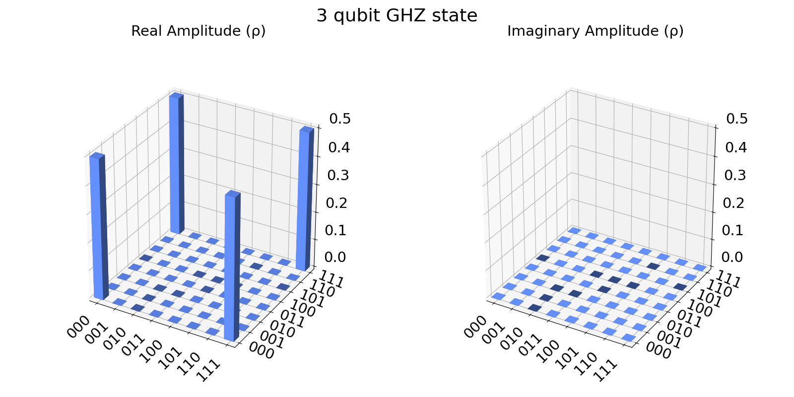
If we remove the shots parameter, we can obtain the statevector

result = backend.run(qc).result()
statevector = result.get_statevector()

# Visualization
plot_state_city(statevector, title="3 qubit GHZ state")
plt.show()

Primitives examples

The current release v0.1.0 introduces several interfaces:

• QulacsEstimator allows users to quickly compute the expectation values of observables using Qulacs’ get_expectation_value.
• QulacsSampler is useful for sampling purposes and uses Qulacs’ QuantumState.

Defining these primitives makes it easy to integrate Qiskit-Qulacs with Qiskit and its extensions. Let’s see an example demonstrating the usage of QulacsEstimator and QulacsSampler. Also, check out the tutorial on the same in Qiskit-Qulacs documentation.

import matplotlib.pyplot as plt
import numpy as np
from qiskit.circuit.library import RealAmplitudes
from qiskit.quantum_info import SparsePauliOp
from qiskit.visualization import plot_histogram

from qiskit_qulacs.qulacs_estimator import QulacsEstimator
from qiskit_qulacs.qulacs_sampler import QulacsSampler

np.random.seed(0)

# Create a circuit, an observable and parameters
num_qubits = 3
qc = RealAmplitudes(num_qubits).decompose()
obs = SparsePauliOp.from_list([("Z" * num_qubits, 1)])
params = np.random.uniform(low=-np.pi, high=np.pi, size=qc.num_parameters)

# Initialize Qulacs Estimator
qulacs_estimator = QulacsEstimator()

# Compute expectation value
result = qulacs_estimator.run([qc], [obs], [params]).result()
print(f"Expectation value: {result.values[0]:.4f}")  # Output: 0.7954

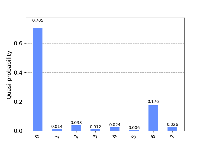
# Obtain Quasi distribution
qc.measure_all()
qulacs_sampler = QulacsSampler()
result = qulacs_sampler.run([qc], [params]).result()

plot_histogram(result.quasi_dists[0])
plt.show()

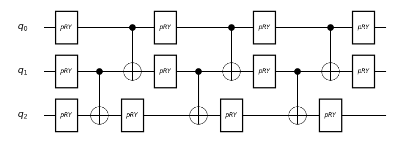
Circuit Visualization

Due to abstraction, the converted circuits are not directly available but are stored as the class’s non-public attribute. We can use qulacs-visualizer to draw the qulacs circuit.

from qulacsvis import circuit_drawer

qc = qulacs_estimator._circuits[0]
qulacs_circuit, _ = qc(params)

circuit_drawer(qulacs_circuit, "mpl")
plt.show()

Gradients

The class QulacsEstimatorGradient uses efficiently Qulacs’ backprop method to compute gradients efficiently. It is enhanced with sympy to support Qiskit’s ParameterExpression which is not natively supported in Qulacs. The below example uses $\theta^2 + \cos\theta$ an in input to the $R_x$ gate.

import numpy as np
from qiskit import QuantumCircuit
from qiskit.circuit import Parameter
from qiskit.quantum_info import SparsePauliOp

from qiskit_qulacs.qulacs_estimator_gradient import QulacsEstimatorGradient

np.random.seed(0)

# Create a circuit, an observable and parameters
theta = Parameter("θ")
theta_val = [0.4]

qc = QuantumCircuit(1)
qc.rx(theta**2 + np.cos(theta), 0)

obs = SparsePauliOp.from_list([("Z", 1)])

# Compute gradients
qulacs_gradient = QulacsEstimatorGradient()
result = qulacs_gradient.run([qc], [obs], [theta_val]).result()
print(f"Gradient: {result.gradients[0][0]:.4f}")  # Output: -0.3623

VQE with Qiskit-Qulacs

We will use the Qiskit-Qulacs primitives and gradients to compute the electronic ground state energy of $H_2$ molecule. Instead of implementing VQE from scratch, we use the VQE class from qiskit-algorithms and demonstrate the capabilities of Qiskit-Qulacs.

from qiskit import transpile
from qiskit_algorithms.minimum_eigensolvers import VQE
from qiskit_algorithms.optimizers import L_BFGS_B
from qiskit_algorithms.utils import algorithm_globals
from qiskit_nature.second_q.algorithms import GroundStateEigensolver
from qiskit_nature.second_q.circuit.library import UCCSD, HartreeFock
from qiskit_nature.second_q.drivers import PySCFDriver
from qiskit_nature.second_q.mappers import JordanWignerMapper

from qiskit_qulacs.qulacs_backend import QulacsBackend
from qiskit_qulacs.qulacs_estimator import QulacsEstimator
from qiskit_qulacs.qulacs_estimator_gradient import QulacsEstimatorGradient

algorithm_globals.random_seed = 42

# Define the molecular system
driver = PySCFDriver(atom="H 0 0 0; H 0 0 0.735", basis="sto3g")
problem = driver.run()
mapper = JordanWignerMapper()  # Qubit Mapper

# Variational form
ansatz = UCCSD(
    problem.num_spatial_orbitals,
    problem.num_particles,
    mapper,
    initial_state=HartreeFock(
        problem.num_spatial_orbitals,
        problem.num_particles,
        mapper,
    ),
)

# Transpile for simulator
transpiled_ansatz = transpile(ansatz, QulacsBackend())

# We set the global phase to zero as qulacs does not supports
# computing its hermitian conjugate which is needed
# during gradient compuatation.
transpiled_ansatz.global_phase = 0.0

# The solver
vqe_solver = VQE(
    QulacsEstimator(),
    transpiled_ansatz,
    L_BFGS_B(),
    gradient=QulacsEstimatorGradient(),
)

# The calculation and results
calc = GroundStateEigensolver(mapper, vqe_solver)
res = calc.solve(problem)

print(f"Electronic ground state energy (Ha): {res.eigenvalues[0]:.4f}")  # -1.8573

Conclusion

Qiskit-Qulacs integrates the Qulacs’ simulator with Qiskit quantum computing framework. Additionally, the library includes source code for benchmarking the execution time with varying qubits. The plots can be found in the documentation and the corresponding code in the benchmarks directory.

For more information, tutorials, and documentation, explore the following links:

• Repository.
• Documentation.
• PyPi.
• Progress documented in the microgrant duration for Phase I and II.

We extend our gratitude to the Unitary Fund for supporting this project with the microgrant program, and we’re excited to be part of the Qiskit Ecosystem. Feel free to reach out to me on LinkedIn if you have any questions or comments.